Majuro Atoll (Republic of the Marshall Islands)
# os
import os
import os.path as op
import sys

# arrays
import math
import numpy as np
import pandas as pd
from scipy import signal as sg

# plot
import matplotlib.pyplot as plt

sys.path.insert(0, os.path.join(os.getcwd()  , '..', '..', '..'))

# dependencies
if(os.path.isdir('waves-main')): #thebe
    os.chdir('waves-main')
from lib.eta_spec import *
import warnings
warnings.filterwarnings("ignore")
warnings.simplefilter('ignore', np.RankWarning)
# path to data
if(os.path.isdir('data')):
    p_data = op.abspath(op.join(os.getcwd(), 'data', 'Majuro')) # thebe
else:
    p_data = op.abspath(op.join(os.getcwd(),'..', '..', '..', 'data', 'Majuro')) # notebook

p_pressure = op.join(p_data, 'Pressure')
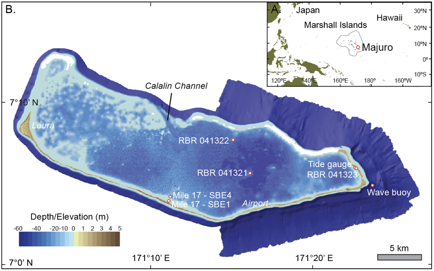
For this study, 1-second data were collected from four pressure sensors deployed during the winter season of 2016-2017 (from mid-November until early February) by Murray Ford (University of Auckland). These pressure sensors were located in the lagoon as shown in the figure bellow; sensors 41320 (tidal gauge) and 41323 were placed closely at the east-side lagoon shoreline, 41321 is situated in the middle of the lagoon and 41322 in front of the shipping channel
Majuro lagoon and pressure sensors location (Ford et al. 2018)
Load data
# Murray sensors  -->  sea pressure (1-sec data)
#xds_41320p = xr.open_dataset(p_pressure + '/Data_41320_pressure')
xds_41321p = xr.open_dataset(p_pressure + '/Data_41321_pressure')
#xds_41322p = xr.open_dataset(p_pressure + '/Data_41322_pressure')
#xds_41323p = xr.open_dataset(p_pressure + '/Data_41323_pressure')
A.1 Observations
sensor = xds_41321p
fig, axs = plt.subplots(2, 1, figsize=(13,10))
axs[0].plot(sensor.time, sensor.Depth, color='b')
axs[1].plot(sensor.time, sensor.Depth, color='b')

axs[0].set_xlabel('Time (1s sampling interval)')
axs[0].set_ylabel('$\eta$ (m)')

axs[1].set_xlabel('Time (1s sampling interval)')
axs[1].set_ylabel('$\eta$ (m)')

axs[0].set_xlim([sensor.time.values[0], sensor.time.values[-1]])
axs[1].set_xlim([sensor.time.values[0], sensor.time.values[100000]])
plt.show()
print("Mean:              ", np.mean(sensor.Depth.values))
print("Standar Deviation: ", np.var(sensor.Depth.values))
Mean:               2.6380446707445464
Standar Deviation:  0.185952843311758
A.2. Spectral Analysis
# Calculate spectra help(sg.welch)
f, E = sg.welch(sensor.Depth, fs = 1, nfft=4*1024)
# Plot wave spectrum
plt.figure(figsize=(5,5))
plt.loglog(f, E, c='b')
plt.xlabel('frequency (Hz)')
plt.ylabel('Densidad espectral (/Hz)')
plt.ylabel('PSD (m²/Hz)')
plt.show()
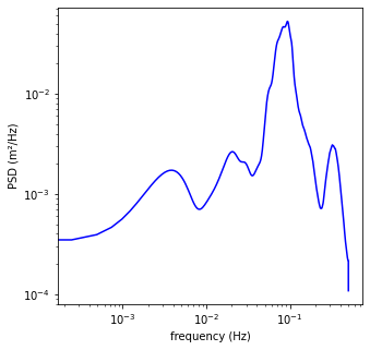
print('Peak frequency: ' + str(f[np.argmax(E)]))
print('Peak period:    ' + str(1/f[np.argmax(E)]))
Peak frequency: 0.093505859375
Peak period:    10.694516971279374
# Eliminate lowest-frequency spectral energy
Es = E[np.where(f > (1/30))[0]]
fs = f[np.where(f > (1/30))[0]]

Ei = E[np.where((f > (1/(5*60))) & (f < (1/30)))[0]]
fi = f[np.where((f > (1/(5*60))) & (f < (1/30)))[0]]
# Plot short-waves spectrum
plt.figure(figsize=(5,5))
plt.plot(fs, Es, c='b', label='Gravity waves', zorder=1)
plt.plot(fi, Ei, c='yellowgreen', label='Infragravity waves', zorder=2)

plt.xlabel('frequency (Hz)')
plt.ylabel('Densidad espectral (/Hz)')
plt.ylabel('PSD (m²/Hz)')
plt.legend()
plt.show()
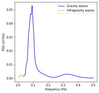
print('Peak frequency: ' + str(fs[np.argmax(Es)]))
print('Peak period:    ' + str(1/fs[np.argmax(Es)]))
Peak frequency: 0.093505859375
Peak period:    10.694516971279374
JONSWAP Goda (1985)
\(S(f)=\alpha\cdot H_{s}^{2} \cdot T_{p}^{-4} \cdot f^{-5} \cdot e^{-1.25 \cdot (T_{p} \cdot f)^{-4}} \cdot \gamma^{e^{-(T_{p} \cdot f - 1)^{2}/(2 \cdot \sigma^{2})}}\)
\(\alpha \approxeq \frac{0.0624}{0.230+0.0336 \cdot \gamma - 0.185 \cdot (1.9 + \gamma)^{-1}}\)
\( \sigma=\begin{cases} \sigma_{a}; f \leq f_{p} \\ \sigma_{b}; f \geq f_{p} \end{cases} \)
\(\gamma = 1 to 7 (mean 3.3), \sigma_{a}\approxeq0.07, \sigma_{b}\approxeq 0.09\)
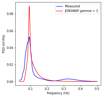
gamma, EJon = assess_jonwsap(fs, Es)
print('Best gamma JONSWAP fit: ' + str(gamma))
Best gamma JONSWAP fit: 3
# Plot measured wave spectrum and theorecial JONSWAP shapes
plt.figure(figsize=(5,5))
plt.plot(fs, Es, c='b', label='Measured')
plt.plot(fs[:-1], EJon, c='r', label='JONSWAP gamma = {0}'.format(gamma))

plt.xlabel('frequency (Hz)')
plt.ylabel('Densidad espectral (/Hz)')
plt.ylabel('PSD (m²/Hz)')
plt.legend()
plt.show()
A.3 Short-term statistics
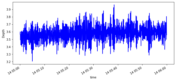
# Select 1 moth
start = '2017-01-14T05:00:00.000000000'
end = '2017-01-14T06:00:00.000000000'
sensor_i = sensor.sel(time=slice(start, end))
sensor_i.Depth.plot(figsize=(10,4), c='b')
plt.show()
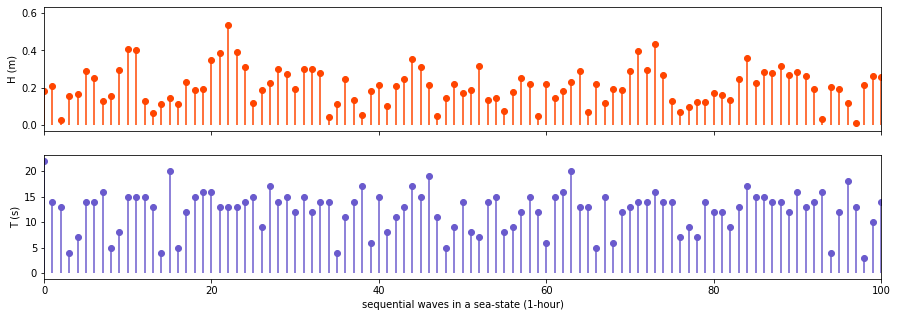
samp = 1
T, H = upcrossing(sensor_i.Depth.values, samp)
fig, axs = plt.subplots(2, 1, figsize=(15,5), sharex=True)
axs[0].vlines(range(len(H)), np.full(len(H), 0), H, color='orangered')
axs[1].vlines(range(len(T)), np.full(len(T), 0), T, color='slateblue')
axs[0].scatter(range(len(H)), H, color='orangered')
axs[1].scatter(range(len(T)), T, color='slateblue')

axs[0].set_ylabel('H (m)')
axs[1].set_ylabel('T (s)')
axs[1].set_xlabel('sequential waves in a sea-state (1-hour)')

plt.xlim(0, 100)
plt.show()
Statistical parameters
mean wave heigh \(\overline H\)
\(\overline H = \frac{1}{N} \sum_{i=1}^{N} H_{i}\)
where i is the sequence number (in time) of the wave in the record
root-mean-square wave height \(H_{rms}\)
\(H_{rms}=(\frac{1}{N} \sum_{i=1}^{N} H_{i}^{2})^{1/2}\)
significant wave heigh \(H_{1/3}\)
\(H_{1/3}=\frac{1}{N/3} \sum_{j=1}^{N/3} H_{j}\)
where j is the rank number of the wave, based on wave-heigh
mean of the highest one-tenth of waves \(H_{1/10}\)
\(H_{1/10}=\frac{1}{N/10} \sum_{j=1}^{N/10} H_{j}\)
mean zero-crossing wave period \(\overline T_{0}\)
\(\overline T_{0}=\frac{1}{N} \sum_{i=1}^{N} T_{0,i}\)
significant wave period \(T_{1/3}\)
\(T_{1/3}=\frac{1}{N/3} \sum_{j=1}^{N/3} T_{0,j}\)
# mean wave heigh
print("mean wave heigh:                        " + str(np.mean(H)))

# root-mean-square wave height
print("root-mean-square wave height:           " + str(rmsV(H)))

# significant wave heigh
print("significant wave heigh:                 " + str(highestN_stats(H, 3)))

# mean of the highest one-tenth of waves
print("mean of the highest one-tenth of waves: " + str(highestN_stats(H, 10)))

# maximun wave heigh
print("maximun wave heigh:                     " + str(np.max(H)))

# mean period
print("mean period:                            " + str(np.mean(T)))

# significant wave period
print("significant wave period:                " + str(highestN_stats(T, 3)))

# mean zero-crossing wave period
print("mean zero-crossing wave period:         " + str(highestN_stats(T, 10)))

# maximun wave period
print("maximun wave period:                    " + str(np.max(T)))
mean wave heigh:                        0.22453318954172838
root-mean-square wave height:           0.2569251425726257
significant wave heigh:                 0.36802250309390466
mean of the highest one-tenth of waves: 0.4832906223671765
maximun wave heigh:                     0.6027064883586348
mean period:                            11.93645484949833
significant wave period:                15.949494949494992
mean zero-crossing wave period:         17.79310344827595
maximun wave period:                    22.000000000000007
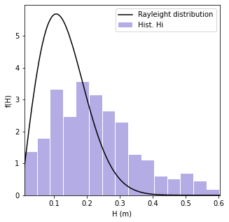
Wave Heigh Distribution
# Rayleigh distribution of individual wave heighs
fHs = [4.01 * (i/(4 * math.sqrt(moment(0, fs, Es)))**2) * np.exp(-2.005 * (i**2/(4 * np.sqrt(moment(0, fs, Es)))**2)) for i in H]
FHs = [1 - np.exp(-2.005 * (i**2/(4 * np.sqrt(moment(0, fs, Es)))**2)) for i in H]
# Plot - sort arrays
plt.figure(figsize=(5,5))
plt.hist(H, density = True, bins = 15, rwidth=0.95, color = "slateblue", alpha=0.5, label='Hist. Hi')
plt.plot(np.sort(H), np.array(fHs)[np.array(H).argsort()], c = "k", zorder = 10, label='Rayleight distribution')

plt.xlabel('H (m)')
plt.ylabel('f(H)')
plt.legend()
plt.xlim(np.nanmin(H), np.nanmax(H))
plt.show()